hlabud usage examples • hlabud

Introduction

Kamil Slowikowski

2024-05-15

hlabud is an R package that provides functions to facilitate download and analysis of human leukocyte antigen (HLA) genotype sequence alignments from IMGTHLA in R.

Let’s consider a question that we might want to answer about HLA genotypes.

What amino acid positions are different between two genotypes?

library(hlabud)
a <- hla_alignments("DRB1")
a$release
#> [1] "3.56.0"
dosage(a$onehot, c("DRB1*03:01:05", "DRB1*03:02:03"))
#>               F26 Y26 D28 E28 F47 Y47 G86 V86
#> DRB1*03:01:05   0   1   1   0   1   0   0   1
#> DRB1*03:02:03   1   0   0   1   0   1   1   0

What nucleotides are different?

n <- hla_alignments("DRB1", type = "nuc")
n$release
#> [1] "3.56.0"
dosage(n$onehot, c("DRB1*03:01:05", "DRB1*03:02:03"))
#>               A164 T164 C171 G171 A227 T227 A240 G240 G344 T344 G345 T345 A357
#> DRB1*03:01:05    1    0    1    0    0    1    1    0    0    1    1    0    1
#> DRB1*03:02:03    0    1    0    1    1    0    0    1    1    0    0    1    0
#>               G357
#> DRB1*03:01:05    0
#> DRB1*03:02:03    1

Installation

The quickest way to get hlabud is to install from GitHub:

# install.packages("devtools")
devtools::install_github("slowkow/hlabud")

Below, I included a few usage examples. I hope they inspire you to share your own HLA analyses.

The source code for this page is available here.

Thank you for reporting issues with hlabud.

Get a one-hot encoded matrix for all HLA-DRB1 alleles

We can use hla_alignments("DRB1") to load the DRB1_prot.txt file from the latest IMGTHLA release:

library(hlabud)
a <- hla_alignments(gene = "DRB1", verbose = TRUE)
#> Reading /home/runner/.local/share/hlabud/3.56.0/alignments/DRB1_prot.txt

The a object is a list with three items:

str(a)
#> List of 7
#>  $ sequences: Named chr [1:3671] "MVCLKLPGGSCMTALTVTLMVLSSPLALAGDTRPRFLWQLKFECHFFNGTERVR.LLERCIYNQEE.SVRFDSDVGEYRAVTELGRPDAEYWNSQKDLLEQRRAAVDTYCR"| __truncated__ "------------------------------------------------------.-----------.--------------------------------------------"| __truncated__ "------------------------------------------------------.-----------.--------------------------------------------"| __truncated__ "------------------------------------------------------.-----------.--------------------------------------------"| __truncated__ ...
#>   ..- attr(*, "names")= chr [1:3671] "DRB1*01:01:01:01" "DRB1*01:01:01:02" "DRB1*01:01:01:03" "DRB1*01:01:01:04" ...
#>  $ alleles  : chr [1:3671, 1:288] "M" "M" "M" "M" ...
#>   ..- attr(*, "dimnames")=List of 2
#>   .. ..$ : chr [1:3671] "DRB1*01:01:01:01" "DRB1*01:01:01:02" "DRB1*01:01:01:03" "DRB1*01:01:01:04" ...
#>   .. ..$ : chr [1:288] "n29" "n28" "n27" "n26" ...
#>  $ onehot   : num [1:3671, 1:1658] 0 0 0 0 0 0 0 0 0 0 ...
#>   ..- attr(*, "dimnames")=List of 2
#>   .. ..$ : chr [1:3671] "DRB1*01:01:01:01" "DRB1*01:01:01:02" "DRB1*01:01:01:03" "DRB1*01:01:01:04" ...
#>   .. ..$ : chr [1:1658] "n29unk" "Mn29" "n28unk" "Ln28" ...
#>  $ gene     : chr "DRB1"
#>  $ type     : chr "prot"
#>  $ release  : chr "3.56.0"
#>  $ file     : chr "/home/runner/.local/share/hlabud/3.56.0/alignments/DRB1_prot.txt"

a$sequences has amino acid sequence alignments in a named character vector:

substr(head(a$sequences, 6), 1, 50)
#>                                     DRB1*01:01:01:01 
#> "MVCLKLPGGSCMTALTVTLMVLSSPLALAGDTRPRFLWQLKFECHFFNGT" 
#>                                     DRB1*01:01:01:02 
#> "--------------------------------------------------" 
#>                                     DRB1*01:01:01:03 
#> "--------------------------------------------------" 
#>                                     DRB1*01:01:01:04 
#> "--------------------------------------------------" 
#>                                     DRB1*01:01:01:05 
#> "--------------------------------------------------" 
#>                                     DRB1*01:01:01:06 
#> "--------------------------------------------------"

Here are the conventions used for alignments (copied from the EBI help page):

The entry for each allele is displayed in respect to the reference sequences.

Where identity to the reference sequence is present the base will be displayed as a hyphen (-).

Non-identity to the reference sequence is shown by displaying the appropriate base at that position.

Where an insertion or deletion has occurred this will be represented by a period (.).

If the sequence is unknown at any point in the alignment, this will be represented by an asterisk (*).

In protein alignments for null alleles, the ‘Stop’ codons will be represented by a hash (X).

In protein alignments, sequence following the termination codon, will not be marked and will appear blank.

These conventions are used for both nucleotide and protein alignments.

a$alleles has a matrix of amino acids with one column for each position:

a$alleles[1:5,1:40]
#>                  n29 n28 n27 n26 n25 n24 n23 n22 n21 n20 n19 n18 n17 n16 n15
#> DRB1*01:01:01:01 "M" "V" "C" "L" "K" "L" "P" "G" "G" "S" "C" "M" "T" "A" "L"
#> DRB1*01:01:01:02 "M" "V" "C" "L" "K" "L" "P" "G" "G" "S" "C" "M" "T" "A" "L"
#> DRB1*01:01:01:03 "M" "V" "C" "L" "K" "L" "P" "G" "G" "S" "C" "M" "T" "A" "L"
#> DRB1*01:01:01:04 "M" "V" "C" "L" "K" "L" "P" "G" "G" "S" "C" "M" "T" "A" "L"
#> DRB1*01:01:01:05 "M" "V" "C" "L" "K" "L" "P" "G" "G" "S" "C" "M" "T" "A" "L"
#>                  n14 n13 n12 n11 n10 n9  n8  n7  n6  n5  n4  n3  n2  n1  1  
#> DRB1*01:01:01:01 "T" "V" "T" "L" "M" "V" "L" "S" "S" "P" "L" "A" "L" "A" "G"
#> DRB1*01:01:01:02 "T" "V" "T" "L" "M" "V" "L" "S" "S" "P" "L" "A" "L" "A" "G"
#> DRB1*01:01:01:03 "T" "V" "T" "L" "M" "V" "L" "S" "S" "P" "L" "A" "L" "A" "G"
#> DRB1*01:01:01:04 "T" "V" "T" "L" "M" "V" "L" "S" "S" "P" "L" "A" "L" "A" "G"
#> DRB1*01:01:01:05 "T" "V" "T" "L" "M" "V" "L" "S" "S" "P" "L" "A" "L" "A" "G"
#>                  2   3   4   5   6   7   8   9   10  11 
#> DRB1*01:01:01:01 "D" "T" "R" "P" "R" "F" "L" "W" "Q" "L"
#> DRB1*01:01:01:02 "D" "T" "R" "P" "R" "F" "L" "W" "Q" "L"
#> DRB1*01:01:01:03 "D" "T" "R" "P" "R" "F" "L" "W" "Q" "L"
#> DRB1*01:01:01:04 "D" "T" "R" "P" "R" "F" "L" "W" "Q" "L"
#> DRB1*01:01:01:05 "D" "T" "R" "P" "R" "F" "L" "W" "Q" "L"

a$onehot has a one-hot encoded matrix with one column for each amino acid at each position:

a$onehot[1:5,1:25]
#>                  n29unk Mn29 n28unk Ln28 Vn28 n27unk Cn27 n26unk Ln26 n25unk
#> DRB1*01:01:01:01      0    1      0    0    1      0    1      0    1      0
#> DRB1*01:01:01:02      0    1      0    0    1      0    1      0    1      0
#> DRB1*01:01:01:03      0    1      0    0    1      0    1      0    1      0
#> DRB1*01:01:01:04      0    1      0    0    1      0    1      0    1      0
#> DRB1*01:01:01:05      0    1      0    0    1      0    1      0    1      0
#>                  Kn25 Rn25 n24unk Fn24 Ln24 n23unk Pn23 n22unk Gn22 n21unk Cn21
#> DRB1*01:01:01:01    1    0      0    0    1      0    1      0    1      0    0
#> DRB1*01:01:01:02    1    0      0    0    1      0    1      0    1      0    0
#> DRB1*01:01:01:03    1    0      0    0    1      0    1      0    1      0    0
#> DRB1*01:01:01:04    1    0      0    0    1      0    1      0    1      0    0
#> DRB1*01:01:01:05    1    0      0    0    1      0    1      0    1      0    0
#>                  Gn21 n20unk Sn20 n19unk
#> DRB1*01:01:01:01    1      0    1      0
#> DRB1*01:01:01:02    1      0    1      0
#> DRB1*01:01:01:03    1      0    1      0
#> DRB1*01:01:01:04    1      0    1      0
#> DRB1*01:01:01:05    1      0    1      0

What is a one-hot encoded matrix? Here is a simple example to demonstrate the idea:

dat <- data.frame(
  V1 = c("A", "A", "B"),
  V2 = c("B", "B", "B"),
  V3 = c("C", "B", "B"),
  stringsAsFactors = TRUE
)
dat
#>   V1 V2 V3
#> 1  A  B  C
#> 2  A  B  B
#> 3  B  B  B
predict(onehot::onehot(dat), dat)
#>      V1=A V1=B V2=B V3=B V3=C
#> [1,]    1    0    1    0    1
#> [2,]    1    0    1    1    0
#> [3,]    0    1    1    1    0

Convert genotypes to a dosage matrix

Suppose we have some individuals with the following genotypes:

genotypes <- c(
  "DRB1*12:02:02:03,DRB1*12:02:02:03",
  "DRB1*04:174,DRB1*15:152",
  "DRB1*04:56:02,DRB1*15:01:48",
  "DRB1*14:172,DRB1*04:160",
  "DRB1*04:359,DRB1*04:284:02"
)

If we want to run an association test on the amino acid positions, then we need to convert the genotype names to a matrix of allele dosages (e.g., 0, 1, 2).

We can use dosage() to convert each individual’s genotypes to amino acid dosages:

dosage <- dosage(a$onehot, genotypes)
dosage[,1:8]
#>                                   n29unk Mn29 n28unk Vn28 n27unk Cn27 n26unk
#> DRB1*12:02:02:03,DRB1*12:02:02:03      0    2      0    2      0    2      0
#> DRB1*04:174,DRB1*15:152                2    0      2    0      2    0      2
#> DRB1*04:56:02,DRB1*15:01:48            2    0      2    0      2    0      2
#> DRB1*14:172,DRB1*04:160                2    0      2    0      2    0      2
#> DRB1*04:359,DRB1*04:284:02             2    0      2    0      2    0      2
#>                                   Ln26
#> DRB1*12:02:02:03,DRB1*12:02:02:03    2
#> DRB1*04:174,DRB1*15:152              0
#> DRB1*04:56:02,DRB1*15:01:48          0
#> DRB1*14:172,DRB1*04:160              0
#> DRB1*04:359,DRB1*04:284:02           0
dim(dosage)
#> [1]   5 428

Note:

The dosage matrix has one row for each individual and one column for each amino acid at each position. By default, dosage() will discard the columns where all individuals are identical.
If input allele names are truncated to 4-digits or 2-digits (e.g. DRB1*03:01 or DRB1*03), then hlabud will pick the first allele that matches the input allele (e.g. DRB1*03:01:01:01). If you want a specific allele, then you need to provide the full allele name in the input.

Please be careful to check that your data looks the way you expect!

Logistic regression association for amino acid positions

Let’s simulate a dataset with cases and controls to demonstrate one approach for testing which amino acid positions might be associated with cases.

set.seed(2)
n <- 100
d <- data.frame(
  geno = paste(
    sample(rownames(a$onehot), n, replace = TRUE),
    sample(rownames(a$onehot), n, replace = TRUE),
    sep = ","
  ),
  age = sample(21:100, n, replace = TRUE),
  case = sample(0:1, n, replace = TRUE)
)
d <- cbind(d, dosage(a$onehot, d$geno))
d[1:5,1:6]
#>                                                          geno age case n29unk
#> DRB1*04:243,DRB1*15:01:01:08     DRB1*04:243,DRB1*15:01:01:08  67    0      1
#> DRB1*04:08:01:01,DRB1*04:56:02 DRB1*04:08:01:01,DRB1*04:56:02  38    1      1
#> DRB1*13:339,DRB1*04:112               DRB1*13:339,DRB1*04:112  67    0      2
#> DRB1*03:85,DRB1*01:02:10             DRB1*03:85,DRB1*01:02:10  55    0      2
#> DRB1*03:62,DRB1*14:224                 DRB1*03:62,DRB1*14:224  73    1      1
#>                                Mn29 n28unk
#> DRB1*04:243,DRB1*15:01:01:08      1      1
#> DRB1*04:08:01:01,DRB1*04:56:02    1      1
#> DRB1*13:339,DRB1*04:112           0      2
#> DRB1*03:85,DRB1*01:02:10          0      2
#> DRB1*03:62,DRB1*14:224            1      1

Our simulated dataset has 100 individuals, 52 cases and 48 controls. We also have one column for each amino acid position that we might want to test for association with the case variable.

One possible approach for association testing is to use glm() to fit a logistic regression model for each amino acid position. This could reveal if any amino acid position might be associated with the case variable in our simulated dataset.

# prepare column names for use in formulas
ix <- 4:ncol(d)
colnames(d)[ix] <- sprintf("VAR%s", colnames(d)[ix])

# select the amino acid positions that have at least 3 people with dosage > 0
my_as <- names(which(colSums(d[,4:ncol(d)] > 0) >= 3))

# run the association tests
my_glm <- rbindlist(pblapply(my_as, function(my_a) {
  f <- sprintf("case ~ %s", my_a)
  glm(as.formula(f), data = d, family = "binomial") %>%
    parameters(exponentiate = TRUE)
}))

# look at the top hits
my_glm %>%
  arrange(p) %>%
  filter(!Parameter %in% c("(Intercept)")) %>%
  head
#>    Parameter Coefficient        SE    CI     CI_low    CI_high         z
#>       <char>       <num>     <num> <num>      <num>      <num>     <num>
#> 1:    VARF37   3.9529448 2.3501312  0.95 1.35121582 14.6317263  2.311857
#> 2:    VARY60   0.4269585 0.1790904  0.95 0.18053396  0.9458131 -2.028981
#> 3:    VARK98   0.5739907 0.1603272  0.95 0.32635370  0.9824460 -1.987475
#> 4:   VARS104   0.5739907 0.1603272  0.95 0.32635370  0.9824460 -1.987475
#> 5:    VARQ96   0.3253919 0.1886793  0.95 0.08932709  0.9191775 -1.936226
#> 6:   VARS179   0.6085247 0.1617164  0.95 0.35644231  1.0163414 -1.869106
#>    df_error          p
#>       <num>      <num>
#> 1:      Inf 0.02078556
#> 2:      Inf 0.04246025
#> 3:      Inf 0.04686976
#> 4:      Inf 0.04686976
#> 5:      Inf 0.05284007
#> 6:      Inf 0.06160809

The volcano below shows the Odds Ratio and P-value for each amino acid position. The top hits with P < 0.05 are labeled.

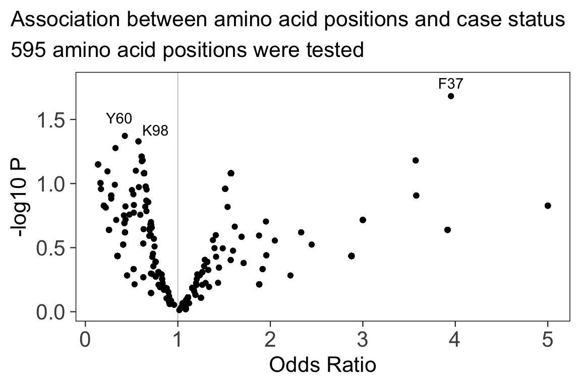
In this simulation, the case variable is associated with F37 (P = 0.021, OR = 4, 95% CI 1.4 to 15).

UMAP embedding of HLA-DRB1 alleles

There are many possibilities for further analysis of the one-hot encoding matrix.

For example, here is a UMAP embedding of HLA-DRB1 alleles encoded as a one-hot amino acid matrix with 1658 columns, one for each amino acid at each position. The color indicates the 2-digit allele name.

uamp(a$onehot, n_epochs = 200, min_dist = 1, spread = 2)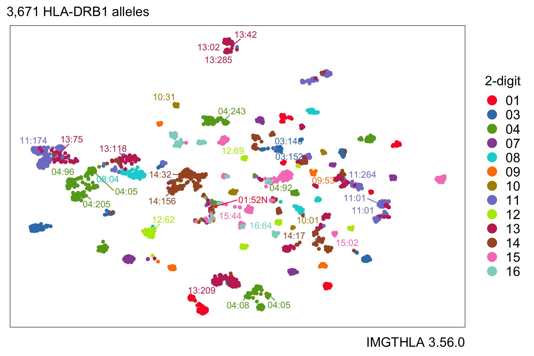

We can highlight which alleles have aspartic acid (Asp or D) at position 57:

Or we can use color to represent the amino acid residue at position 57:

Get HLA allele frequencies from Allele Frequency Net Database (AFND)

The hlabud R package includes a table of HLA allele frequencies from the Allele Frequency Net Database (AFND).

If you use this data, please cite the latest manuscript about Allele Frequency Net Database:

Gonzalez-Galarza FF, McCabe A, Santos EJMD, Jones J, Takeshita L, Ortega-Rivera ND, et al. Allele frequency net database (AFND) 2020 update: gold-standard data classification, open access genotype data and new query tools. Nucleic Acids Res. 2020;48: D783–D788. doi:10.1093/nar/gkz1029

af <- hla_frequencies()
af
#> # A tibble: 123,502 × 7
#>    group gene  allele  population            indivs_over_n alleles_over_2n     n
#>    <chr> <chr> <chr>   <chr>                         <dbl>           <dbl> <dbl>
#>  1 hla   A     A*01:01 Argentina Rosario To…          15.1           0.076    86
#>  2 hla   A     A*01:01 Armenia combined Reg…          NA             0.125   100
#>  3 hla   A     A*01:01 Australia Cape York …          NA             0.053   103
#>  4 hla   A     A*01:01 Australia Groote Eyl…          NA             0.027    75
#>  5 hla   A     A*01:01 Australia New South …          NA             0.187   134
#>  6 hla   A     A*01:01 Australia Yuendumu A…          NA             0.008   191
#>  7 hla   A     A*01:01 Austria                        27             0.146   200
#>  8 hla   A     A*01:01 Azores Central Islan…          NA             0.08     59
#>  9 hla   A     A*01:01 Azores Oriental Isla…          NA             0.115    43
#> 10 hla   A     A*01:01 Azores Terceira Isla…          NA             0.109   130
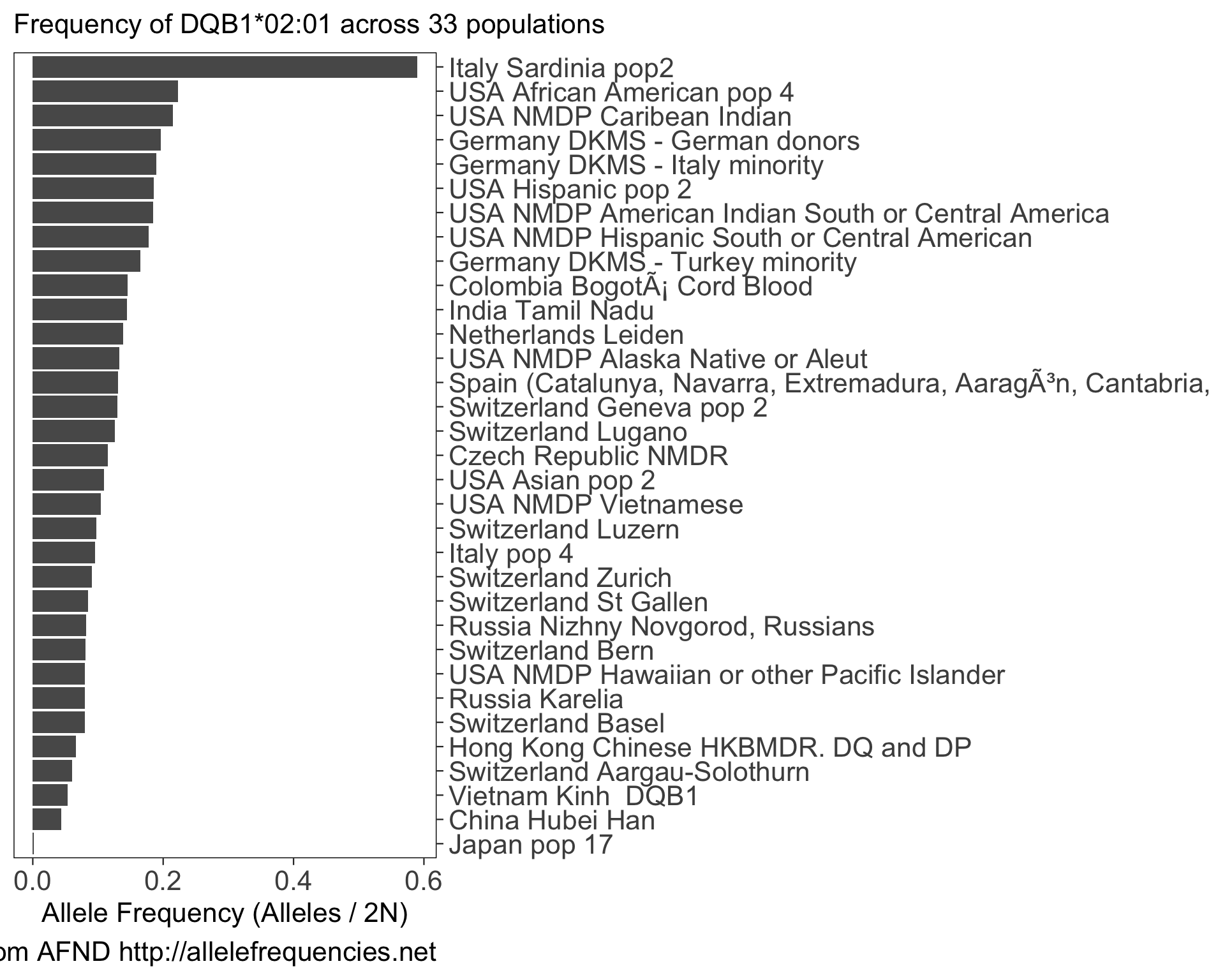
#> # ℹ 123,492 more rows

We can use this data to plot the frequency of a specific allele (e.g. DQB1*02:01) in populations with more than 1000 sampled individuals:

my_allele <- "DQB1*02:01"
my_af <- af %>% filter(allele == my_allele) %>%
  filter(n > 1000) %>%
  arrange(-alleles_over_2n)

ggplot(my_af) +
  aes(x = alleles_over_2n, y = reorder(population, alleles_over_2n)) +
  scale_y_discrete(position = "right") +
  geom_colh() +
  labs(
    x = "Allele Frequency (Alleles / 2N)",
    y = NULL,
    title =  glue("Frequency of {my_allele} across {length(unique(my_af$population))} populations"),
    caption = "Data from AFND http://allelefrequencies.net"
  )

See github.com/slowkow/allelefrequencies for more examples of how we might use this data.

Compute HLA divergence with the Grantham distance matrix

Humans are diploid, so each of us has two copies of each HLA gene. An individual with two highly dissimilar alleles can bind a greater number of different peptides than a homozygous individual (https://doi.org/10.1007/BF02918202):

Each MHC class II allele has the capacity to bind and present a specific set of peptides from processed antigens. The inability of a specific class II allele to bind and present a fragment derived from a processed antigen results in the loss of immune responsiveness for that antigen in individuals homozygous for that class II allele.

The amino acid distance matrix by Granthan 1974 (https://doi.org/10.1126/science.185.4154.862) encodes information about the composition, polarity, and molecular volume of each amino acid.

grantham
#>    amino    c    p     v
#> 1    Ser 1.42  9.2  32.0
#> 2    Arg 0.65 10.5 124.0
#> 3    Leu 0.00  4.9 111.0
#> 4    Pro 0.39  8.0  32.5
#> 5    Thr 0.71  8.6  61.0
#> 6    Ala 0.00  8.1  31.0
#> 7    Val 0.00  5.9  84.0
#> 8    Gly 0.74  9.0   3.0
#> 9    Ile 0.00  5.2 111.0
#> 10   Phe 0.00  5.2 132.0
#> 11   Tyr 0.20  6.2 136.0
#> 12   Cys 2.75  5.5  55.0
#> 13   His 0.58 10.4  96.0
#> 14   Gln 0.89 10.5  85.0
#> 15   Asn 1.33 11.6  56.0
#> 16   Lys 0.33 11.3 119.0
#> 17   Asp 1.38 13.0  54.0
#> 18   Glu 0.92 12.3  83.0
#> 19   Met 0.00  5.7 105.0
#> 20   Trp 0.13  5.4 170.0

We can use that matrix to compute an HLA divergence metric for a set of individuals like this:

my_genos <- c("A*23:01:12,A*24:550", "A*25:12N,A*11:27", "A*24:381,A*33:85")

hla_divergence(my_genos)
#> A*23:01:12,A*24:550    A*25:12N,A*11:27    A*24:381,A*33:85 
#>           0.5131579           3.4736842           5.1078947

The divergence for a homozygote is equal to zero, by definition:

hla_divergence("A*01:01,A*01:01")
#> A*01:01,A*01:01 
#>               0

hlabud includes R code for the divergence calculations that was translated from the original Perl code by Pierini & Lenz 2018 (https://doi.org/10.1093/molbev/msy116).

The amino acid distance matrix is easily accessible, and we provide two built-in options “grantham” and “uniform”:

amino_distance_matrix(method = "grantham")
#>     A   R   N   D   C   Q   E   G   H   I   L   K   M   F   P   S   T   W   Y
#> A   0 112 111 126 195  91 107  60  86  94  96 106  84 113  27  99  58 148 112
#> R 112   0  86  96 180  43  54 125  29  97 102  26  91  97 103 110  71 101  77
#> N 111  86   0  23 139  46  42  80  68 149 153  94 142 158  91  46  65 174 143
#> D 126  96  23   0 154  61  45  94  81 168 172 101 160 177 108  65  85 181 160
#> C 195 180 139 154   0 154 170 159 174 198 198 202 196 205 169 112 149 215 194
#> Q  91  43  46  61 154   0  29  87  24 109 113  53 101 116  76  68  42 130  99
#> E 107  54  42  45 170  29   0  98  40 134 138  56 126 140  93  80  65 152 122
#> G  60 125  80  94 159  87  98   0  98 135 138 127 127 153  42  56  59 184 147
#> H  86  29  68  81 174  24  40  98   0  94  99  32  87 100  77  89  47 115  83
#> I  94  97 149 168 198 109 134 135  94   0   5 102  10  21  95 142  89  61  33
#> L  96 102 153 172 198 113 138 138  99   5   0 107  15  22  98 145  92  61  36
#> K 106  26  94 101 202  53  56 127  32 102 107   0  95 102 103 121  78 110  85
#> M  84  91 142 160 196 101 126 127  87  10  15  95   0  28  87 135  81  67  36
#> F 113  97 158 177 205 116 140 153 100  21  22 102  28   0 114 155 103  40  22
#> P  27 103  91 108 169  76  93  42  77  95  98 103  87 114   0  74  38 147 110
#> S  99 110  46  65 112  68  80  56  89 142 145 121 135 155  74   0  58 177 144
#> T  58  71  65  85 149  42  65  59  47  89  92  78  81 103  38  58   0 128  92
#> W 148 101 174 181 215 130 152 184 115  61  61 110  67  40 147 177 128   0  37
#> Y 112  77 143 160 194  99 122 147  83  33  36  85  36  22 110 144  92  37   0
#> V  64  96 133 152 192  96 121 109  84  29  32  97  21  50  68 124  69  88  55
#>     V
#> A  64
#> R  96
#> N 133
#> D 152
#> C 192
#> Q  96
#> E 121
#> G 109
#> H  84
#> I  29
#> L  32
#> K  97
#> M  21
#> F  50
#> P  68
#> S 124
#> T  69
#> W  88
#> Y  55
#> V   0

Download and unpack all data from the latest IMGTHLA release

If you only want to use hla_alignments(), then you don’t need install_hla() because data files are downloaded automatically as needed and cached for future use.

But some users might need access to additional files that are only present in the full data release.

Run install_hla() to download and unpack the latest IMGTHLA release. The destination folder for the downloaded data files is getOption("hlabud_dir") (automatically tailored to your operating system thanks to the rappdirs package).

Here are a few examples of how to download releases or get a list of release names.

Download the latest release (default) or a specific release:

# Download all of the data (120MB) for the latest IMGTHLA release
install_hla(release = "latest")

# Download a specific release
install_hla(release = "3.51.0")

Optionally, get or set the directory hlabud uses to store the data:

getOption("hlabud_dir")
#> [1] "/home/username/.local/share/hlabud"

# Manually override the directory for hlabud to use
options(hlabud_dir = "/path/to/my/dir")

After installing a few releases, the hlabud folder might look like this:

❯ ls -lah "/home/user/.local/share/hlabud"
total 207M
drwxrwxr-x  3 user user      32 Apr  5 01:19 3.30.0
drwxrwxr-x 11 user user    4.0K Apr  7 19:31 3.40.0
drwxrwxr-x 12 user user    4.0K Apr  5 00:27 3.51.0
-rw-rw-r--  1 user user     15K Apr  7 19:23 tags.json
-rw-rw-r--  1 user user     79M Apr  7 19:28 v3.40.0-alpha.tar.gz
-rw-rw-r--  1 user user    129M Apr  4 20:07 v3.51.0-alpha.tar.gz

Count the number of alleles in each IMGTHLA release

We can get a list of the release names:

releases <- hla_releases()
releases
#>  [1] "3.56.0"   "3.55.0"   "3.54.0"   "3.53.0"   "3.52.0"   "3.51.0"  
#>  [7] "3.50.0"   "3.49.0"   "3.48.0"   "3.47.0"   "3.46.0"   "3.45.1"  
#> [13] "3.45.01"  "3.45.0.1" "3.45.0"   "3.44.1"   "3.44.0"   "3.43.0"  
#> [19] "3.42.0"   "3.41.2"   "3.41.0"   "3.40.0"   "3.39.0"   "3.38.0"  
#> [25] "3.37.0"   "3.36.0"   "3.35.0"   "3.34.0"   "3.33.0"   "3.32.0"

Then we can get the allele names for each release:

my_alleles <- rbindlist(lapply(releases, function(release) {
  retval <- hla_alleles(release = release)
  retval$release <- release
  return(retval)
}), fill = TRUE)
#> Warning in hla_alleles(release = release): unrecognized release name
#> 'Allelelist.3451.txt'
#> Warning in hla_alleles(release = release): unrecognized release name
#> 'Allelelist.34501.txt'
#> Warning in hla_alleles(release = release): unrecognized release name
#> 'Allelelist.34501.txt'
#> Warning in hla_alleles(release = release): unrecognized release name
#> 'Allelelist.3441.txt'
#> Warning in hla_alleles(release = release): unrecognized release name
#> 'Allelelist.3412.txt'

Next, count how many alleles we have in each release:

d <- my_alleles %>% count(release) %>% filter(n > 1)
d
#>     release     n
#>      <char> <int>
#>  1:  3.32.0 18363
#>  2:  3.33.0 18955
#>  3:  3.34.0 20272
#>  4:  3.35.0 21683
#>  5:  3.36.0 22548
#>  6:  3.37.0 24093
#>  7:  3.38.0 25958
#>  8:  3.39.0 26512
#>  9:  3.40.0 27273
#> 10:  3.41.0 27980
#> 11:  3.42.0 28786
#> 12:  3.43.0 29417
#> 13:  3.44.0 30523
#> 14:  3.45.0 31552
#> 15:  3.46.0 32330
#> 16:  3.47.0 33552
#> 17:  3.48.0 34145
#> 18:  3.49.0 35077
#> 19:  3.50.0 36016
#> 20:  3.51.0 36625
#> 21:  3.52.0 37068
#> 22:  3.53.0 37619
#> 23:  3.54.0 38416
#> 24:  3.55.0 38909
#> 25:  3.56.0 39886
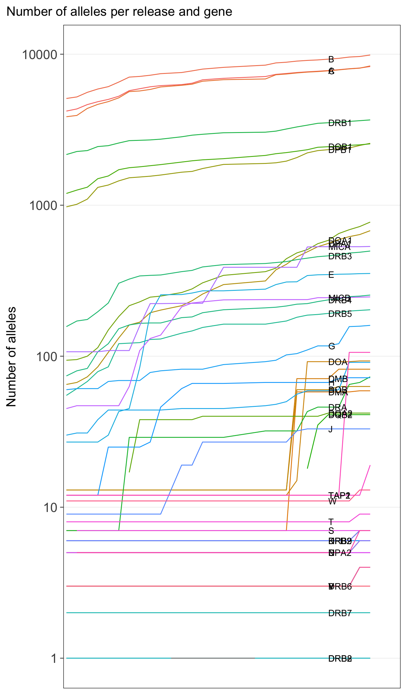
#>     release     n

And plot the number of alleles as a line plot:

ggplot(d) +
  aes(x = release, y = n, group = 1) +
  geom_line() +
  geom_text(aes(label = release), hjust = 1) +
  labs(x = NULL, y = "Number of alleles",
  title = "Each release has more HLA alleles") +
  theme(
    axis.text.x = element_blank(),
    axis.ticks.x = element_blank(),
  )

d2 <- my_alleles %>% mutate(gene = str_split_fixed(Allele, "\\*", 2)[,1]) %>% count(release, gene)
ggplot() +
  aes(x = release, y = n) +
  geom_line(
    data = d2,
    aes(group = gene, color = gene)
  ) +
  scale_color_discrete(guide = "none") +
  geom_text(
    data = d2 %>% filter(release == "3.52.0"),
    mapping = aes(label = gene),
    hjust = 0
  ) +
  labs(x = NULL, y = "Number of alleles",
  title = "Number of alleles per release and gene") +
  scale_x_discrete(expand = expansion(mult = c(0.01, 0.1))) +
  scale_y_log10() +
  theme(
    panel.grid.major.y = element_line(), 
    axis.text.x = element_blank(),
    axis.ticks.x = element_blank(),
  )